Dossier 003 · CubeSat B-Dot Detumbling

1 · Mission Context

CubeSats released from launch vehicles typically begin their operational life with substantial angular velocity. Deployment springs and separation dynamics introduce rotational disturbances that must be damped before precision attitude control can begin.

Small satellites frequently rely on magnetorquers for initial detumbling. By interacting with the Earth's magnetic field these coils generate torques that dissipate rotational kinetic energy.

The objective of this project is to construct a numerical simulation environment capable of evaluating the performance of a magnetic B-Dot detumbling controller.

2 · Spacecraft Attitude Dynamics

The rotational dynamics of the spacecraft are governed by Euler's rigid body equation.

\[ J\dot{\omega} + \omega \times (J\omega) = \tau \]

where

\(J\) — inertia tensor
\(\omega\) — angular velocity vector
\(\tau\) — total external torque

The net torque acting on the spacecraft includes both magnetic control torque and gravity gradient disturbance.

\[ \tau = \tau_{mag} + \tau_{gg} \]

3 · Orbit Propagation

The spacecraft orbit is propagated using the classical two-body gravitational model.

\[ \dot r = v \]

\[ \dot v = -\frac{\mu}{r^3}r \]

where the gravitational parameter of Earth is

\[ \mu = 3.986004418 \times 10^{14} \; m^3/s^2 \]

FIGURE 003-A · ORBIT PROPAGATION

4 · Magnetic Field Model

Magnetorquer actuation relies on the interaction between the spacecraft magnetic dipole and the Earth's magnetic field.

In this simulation the magnetic field is approximated using a dipole model.

\[ B = \frac{\mu_0}{4\pi r^3} \left[ 3(\hat m \cdot \hat r)\hat r - \hat m \right] \]

Typical field magnitudes in low Earth orbit range between 25 and 60 microtesla.

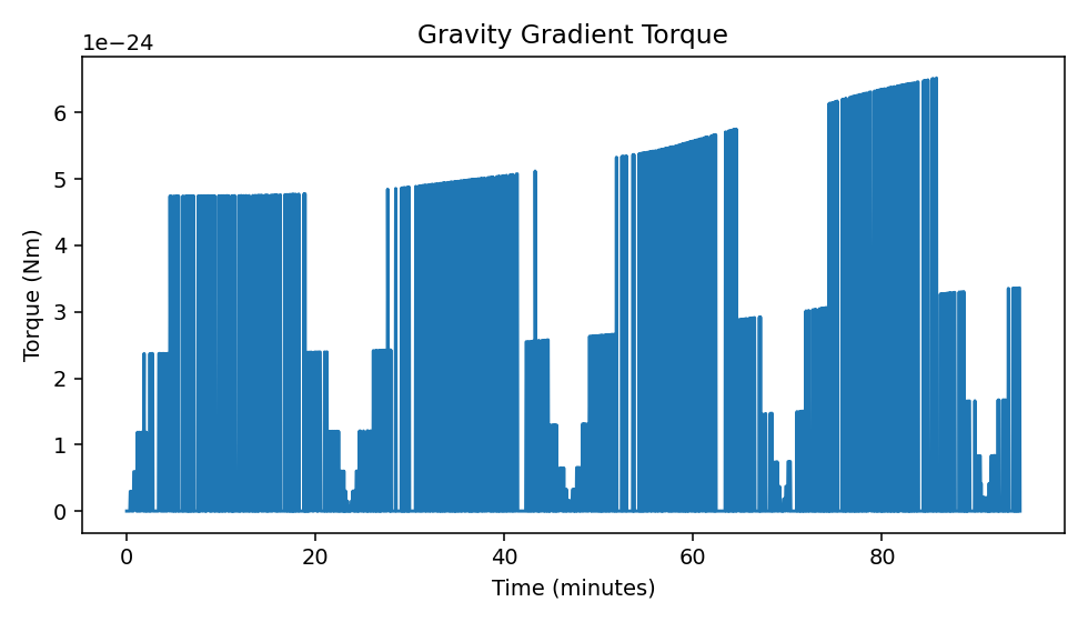
FIGURE 003-B · MAGNETIC FIELD ALONG ORBIT

5 · Gravity Gradient Disturbance

Because Earth’s gravitational field varies across the spacecraft structure, a restoring torque arises whenever the spacecraft inertia axes are misaligned with the radial direction.

\[ \tau_{gg} = \frac{3\mu}{r^5}(r \times Jr) \]

FIGURE 003-C · GRAVITY GRADIENT TORQUE

6 · B-Dot Control Law

The B-Dot controller commands a magnetic dipole moment that opposes the time derivative of the measured magnetic field.

The magnetic field rate is approximated using the spacecraft angular velocity.

\[ \dot B \approx -\omega \times B \]

The control law becomes

\[ m = -k \dot B \]

In this project a bang-bang implementation is used.

\[ m = -m_{max} \; sign(\dot B) \]

7 · Simulation Implementation

The spacecraft dynamics and control law are integrated using the SciPy ODE solver. Each subsystem of the simulation corresponds directly to the governing equations described earlier.

Orbit Dynamics

def orbit_dynamics(t,state):

    r = state[0:3]
    v = state[3:6]

    r_norm = np.linalg.norm(r)

    a = -mu * r / r_norm**3

    return np.hstack((v,a))

This function implements the two-body gravitational equations of motion.

B-Dot Controller

bdot = -np.cross(w,B)

m = -m_max * np.sign(bdot)

The cross product approximates the magnetic field time derivative. The commanded dipole moment is then saturated to the maximum magnetorquer capability.

8 · Detumbling Performance

Simulation results show that the B-Dot controller gradually dissipates rotational kinetic energy, reducing the spacecraft angular velocity over approximately one orbital period.

FIGURE 003-D · ANGULAR RATE DECAY

References

Wertz, J. R. — Spacecraft Attitude Determination and Control
Markley & Crassidis — Fundamentals of Spacecraft Attitude Determination
Psiaki, M. — Magnetic Attitude Control of Satellites
NASA Guidance Navigation and Control Handbook

CUBESAT B-DOT DETUMBLING

Spacecraft

Orbit

Initial Angular Rates